Interpreting Multinomial Logistic Regression in Stata

Author: Bailey DeBarmore

You may find yourself running a multinomial logistic regression, but unsure how to interpret your output. I get these questions alot from students, so I'm here to help demystify your Stata results. 

Running the regression

To run a multinomial logistic regression, you'll use the command -mlogit-. 

You can see the code below that the syntax for the command is mlogit, followed by the outcome variable and your covariates, then a comma, and then base(#).

​In this example I have a 4-level variable, hypertension (htn). I want the reference category, or the base outcome, to be normal BP, which corresponds to htn=0. So I'll use base(0) in my code. 

​*Analysis question: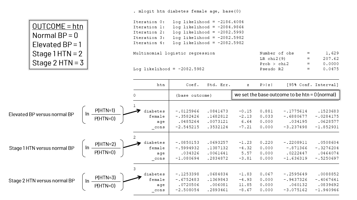 
*Estimate the association of diabetes with hypertension stage
*Adjusting for sex and age
*SYNTAX: mlogit <outcome> <covariates>, base(#)

*the option base(#) allows you tell Stata what level of the outcome variable
*should be the reference - for us we'll make it htn = 0 (normal)
set more off
set line 200

*Run the model

mlogit htn diabetes female age, base(0) 

Figure 1. Stata output from running an mlogit command with a 4-level hypertension outcome, with diabetes, female sex, and age (yrs) as covariates. Each box with repeated covariates corresponds to a level of the outcome compared to the reference (which we indicated in base(#)).

Above is the Stata output from running the mlogit command. 

You can see that there is a box at the top for htn=0, because we set that as the base outcome. If we had set the base outcome to be htn=2, we would have covariate output for 0, 1, and 3, and where the 2 box is, would be a blank with (base outcome). 

Each box corresponds to the estimated log odds of that covariate for one outcome level versus the base outcome. You can see where htn=1, it's estimating P(Elevated BP) vs P(Normal BP) (on the natural log scale). 

The Equations

Let's connect this output with the regression equation. When I want to pull estimates, I often enter in the coefficients to an MS Excel spreadsheet, and knowing how the output translates to the equation is important.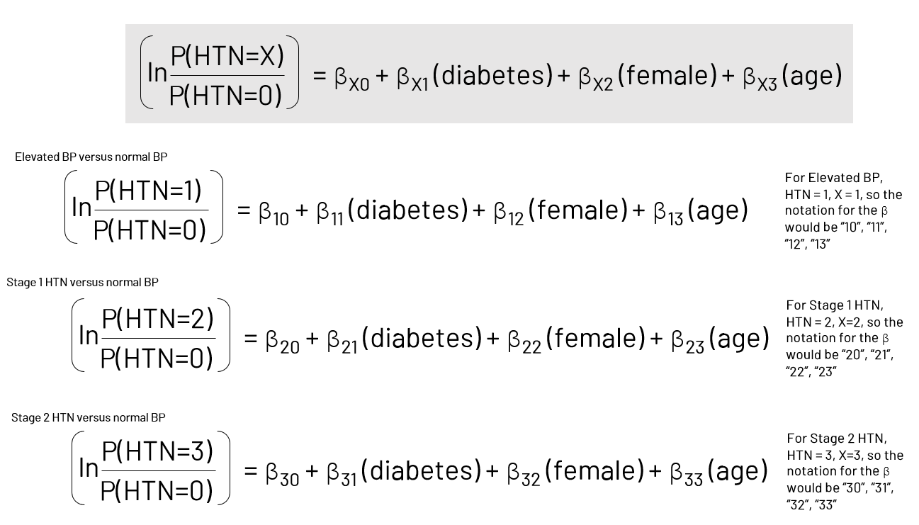

Figure 2. How do we bring our regression output back to the statistical equation? You can write out the equation for each otucome versus the reference, here HTN = 0 or normal BP, with beta (coefficient) subscripts that correspond to the level of the outcome.

Usually we write out the equation with just beta-0, beta-1, beta-2, etc. but since we have multiple levels of the outcome, each coefficient will be prefixed by X, which indicates the level of the variable (gray equation). I have it written out for each HTN level. 

Let's apply it in an example using elevated BP vs normal.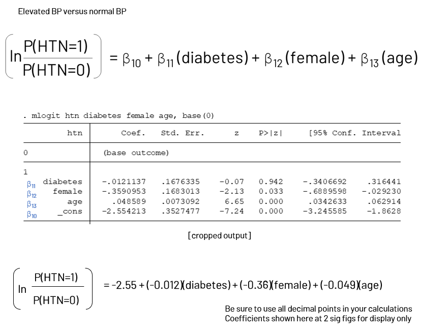

Figure 3. Here's an example calculation where we plug in the coefficients for HTN = 1, elevated BP, into the equation we wrote out in Figure 2.

Helpful Links
​
UCLA Institute for Digital Research and Education

• Annotated Output for Multinomial Logistic Regression in Stata
• Multinomial Logistic Regression in Stata Data Analysis Examples

Stata Documentation for mlogit

Exponentiate

But we are really interested in the exponentiated coefficients, or the relative risk ratio in this scenario. In other Stata regression, we can use the option "or" or "exp" to transform our coefficients into the ratio. With -mlogit-, you do something a bit different - you use the option rrr in a statement run right after your regression and Stata will transform the log odds into the relative probability ratios, or the relative risk ratio (RRR).

*Get exponentiated results;
mlogit htn diabetes female age, base(0) 
mlogit,rrr

*Is the effect of diabetes on Elevated BP vs normal BP similar for Stage 2 HTN vs normal BP?
test [1]diabetes = [3]diabetes

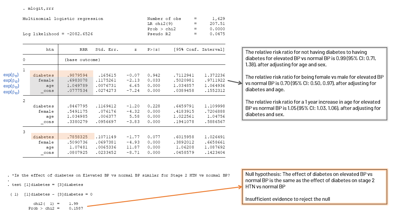Figure 4. To get the relative risk ratio (RRR), we run "mlogit, rrr" after running our regression. In this figure you'll see interpretations of the elevated BP vs normal BP in the grey box, and a test for the effect of diabetes in 2 outcome levels (orange box).

The output format when we run -mlogit, rrr- is the same as before, but we have exponentiated betas.  If you use a calculator and exponentiate the betas in the original output you'll see they match up.  

I've interpreted the RRR for elevated BP vs normal BP in the grey box. 

You may be interested if the effect of one covariate is the same across levels of the outcome. For example, does the effect of diabetes differ when we look at elevated BP vs normal BP versus stage 2 hypertension vs normal BP? 

We can use the test command and indicate the level of the outcome in [ ] 's. 

By writing the test statement out that the values are equal to each other, we are testing the null hypothesis that they are equal, or that their difference is zero. The prob > chi2 gives us the probability of observing a more extreme chi2 value, and here our p-value of 0.16 indicates we won't be rejecting the null this time around -> the effect of diabetes in elevated BP vs normal BP versus stage 2 HTN vs normal BP is similar. 

Marginal Probabilities

Figure 5. You can estimate the predicted probability of diabetes at each level of the outcome, holding the other covariates at their means. Each box corresponds to an outcome level.

If you want to estimate the predicted probability of each outcome for those with adn without diabetes, you can use the margins command. You run the margins command for each level of outcome. Be sure that your factor variable of interest (diabetes in the example) is run in the regression as a factor variable (i.variable). There's usually no need to do this with binary outcomes, so you may not have. Just re-run your regression with i.variable (you can even do so 'quietly') and then run margins. Note that if you want to always run your covariates as factor variables (binary or categorical) you can do so. For a binary variable it will just give you 1.variable for a 0-1 variable, or you can tell Stata you want 1 to be the reference with ib1.variable. 

With the margins command you can set each covariate to a level, such as female=1 (the average sex part here doesn't mean much) or you can predict atmeans (which is useful for age). 

---

About the Author

Bailey DeBarmore is a doctoral student at the University of North Carolina at Chapel Hill studying epidemiology. Find her on Twitter @BaileyDeBarmore and blogging for the American Heart Association on the Early Career Voice blog. ​​​​