Calculating IPW and SMR in SAS

Calculating IPW and SMR in SAS and Stata

4/14/2019

Author: Bailey DeBarmore

Learning about a method in class, like inverse probability weighting, is different than implementing it in practice.

This post will remind you why we might be interested in propensity scores to control for confounding - specifically inverse probability of treatment weights and SMR - and then show how to do so in SAS and Stata.

If you have corresponding code in R that you'd like to add to this post, please contact me.

A note about weighting versus multivariable regression:
Effect estimate interpretations when you use weighting are marginal effect in the target population. When you adjust for covariates in a regression model, you are interpreting a conditional effect, that is, the effect of the exposure holding (conditional on) the covariates being constant.

Conditional estimates are troublesome with time-varying covariates because we run into collider bias and conditioning on mediators, thus weights are preferable. In simpler situations, using weights over multivariable regression can help with convergence issues .

Files to Download: .txt file with SAS and Stata code, as well as a PDF version of this post with code (perfect for students) available to download at the end of the post or at my github

propensity scores

A propensity score is a predicted probability that may be used to predict exposure (or treatment) status, but can also be used for censoring or missingness.

How do we use propensity scores for confounding?
We can use propensity scores to generate WEIGHTS which, when applied to the final model, make the exposure independent from confounders (Figure 1B), usually by modeling the association between the exposure and confounders (instead of the main analysis where we model the outcome and exposure).

Propensity scores can also control for confounding via covariate adjustment (I discourage you from this option), stratification, and matching, in addition to weighting.

The 2 types of weights I'll be discussing in this post are

SMR (standardized mortality/morbidity ratio) weights
IPTW (inverse probability of treatment weights)

Creating a pseudopopulation via propensity scores | EPICODE

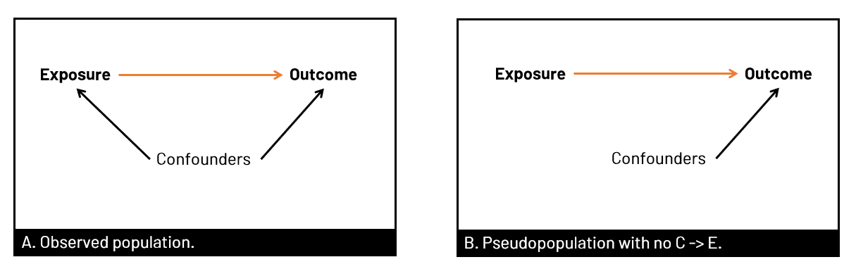Figure 1. Panel A shows the observed population in our data set, where the relationship between exposure and outcome (orange) is confounded by well, confounders. In B, we have removed the arrow from confounders to exposure. We can remove the arrow in several ways, including using propensity scores (of various types) to create a pseudopopulation where the exposure and confounder are no longer associated.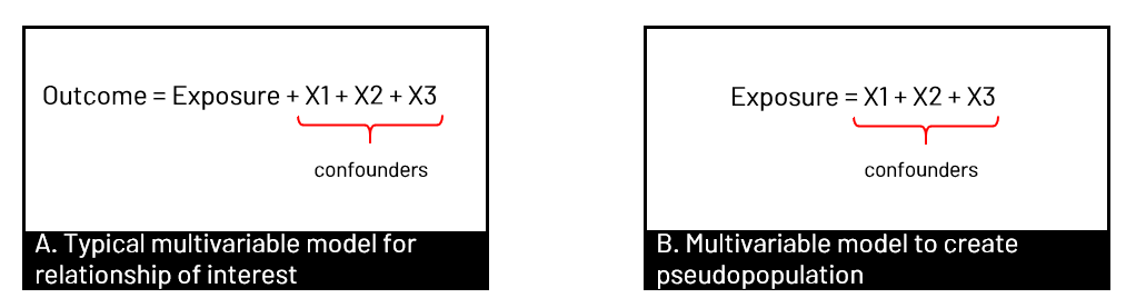

Figure 2. Panel A shows the usual multivariable model we run in our analyses - to estimate the association of the exposure with the outcome, controlled for confounders. When we want to use propensity scores, we first create the weights that we will later use in our final model by modeling the association of the confounders with the exposure - so we can remove that arrow.

SMR

When you use SMR weights, you're estimating the average treatment effect in the treated (ATT). In other words, you estimate the effect had the exposed group been exposed, versus the exposed group been unexposed. The pseudopopulation that you create has a covariate (confounder) distribution equal to that observed in the exposed group.

You can also generate your SMR weights where the unexposed group is the target of interest, and model the effect had the unexposed group been unexposed versus the unexposed group been exposed.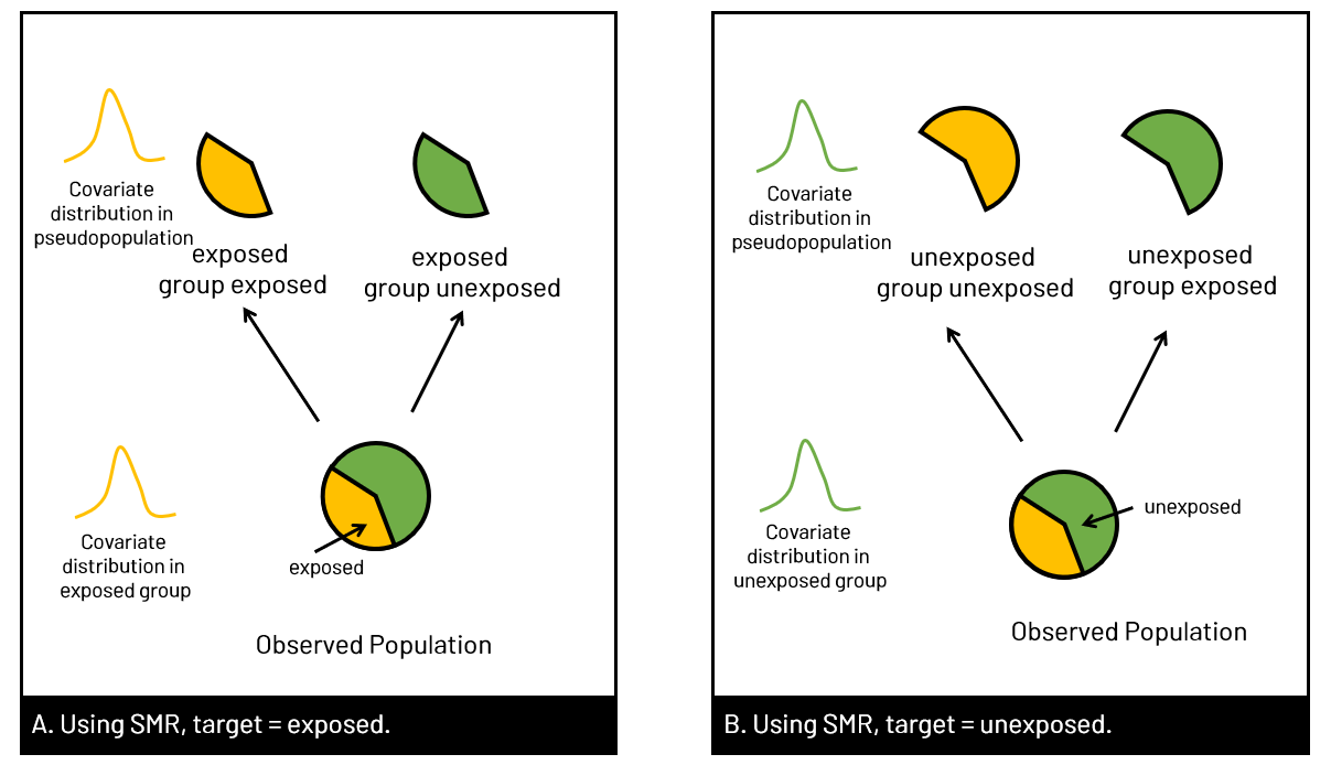

SMR with exposed and unexposed target groups | EPICODE

Figure 3. In Panel A, the target group is the exposed group, so we use SMR to model had the exposed group been exposed versus unexposed, with the covariate distribution of the exposed group (yellow). In Panel B, we use the covariate distribution of the unexposed group (green), and model had unexposed group been unexposed vs exposed.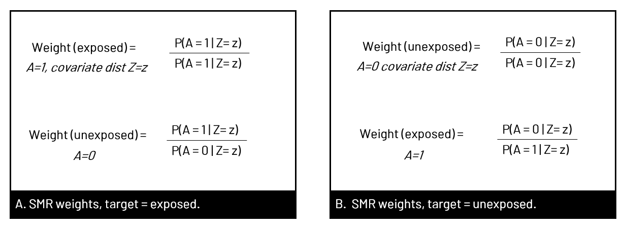

Figure 4. Equations to calculate the SMR weights for given target population corresponding to Figure 3 examples. A indicates exposure status (=1 for exposed, =0 for unexposed). The numerator is the probabilitiy of exposure given the covariate distribution of the target group, and the denominator is the probability of being assigned to what was observed. You can see that in panel B, it switches when the target group is unexposed.

coding SMR in SAS

To use SMR, you'll be generating the probabilities for the numerator and denominator, and then creating the weight (numerator/denominator) and applying it in the appropriate statement.

***********************************************
* Calculating SMR weights where exposure = 0, 1
**************************************(********;

&let data=<data>;
&let y=<outcome>;
&let x=<exposure>;
&let id=<id>;

*Estimate the predicted probability given covariates;

proc logistic data=&data desc;
model &x=<covariates>;
output out=pred p=p1;
run;

*Generate the weights by exposure status, for exposed group = target their weight will be 1;

data <newdata>;
set pred;
p0 = 1-p1;
odds = p1/p0;
if &x=1 then wt=1;
else wt=odds;
run;

*Final weighted analysis;
proc logistic data=<newdata> desc;
weight wt;
model &y = &x;
run;

***********************************************
* Calculating SMR weights where exposure = categorical
**************************************(********;

&let data=<data>;
&let y=<outcome>;
&let x=<exposure>;
&let id=<id>;

*Estimate the predicted probability given covariates;

proc logistic data=&data desc;
model &x=<covariates> /LINK= glogit;
output out=pred p=p1;
run;

*Generate the weights by exposure status, for exposed group = target their weight will be 1;

data <newdata>;
set pred;
p0 = 1-p1;
odds = p1/p0;
if &x=1 then wt=1;
else wt=odds;
run;

*Final weighted analysis;
proc logistic data=<newdata> desc;
weight wt;
model &y = &x;
run;

What is &let?
So that you can easily adapt my code, I use &let statements at the beginning of my code blocks. After the equals sign, you would replace <data> with your dataset name, <exposure> with your exposure variable, and <outcome> with your outcome variable. The code as written will then run with those chosen variables. Note that you do need to replace <covariates> in the model statement with your confounders.

If you don't want to use &let statements, simply go through the code and anywhere you see &<text>, replace both the & and the text with your regular code.

coding SMR in Stata

The approach to calculating SMR is different in Stata. You'll be using the built in teffects command (reference manual [TE] here) and using options to specify SMR versus IPW.

Since using SMR gives us the average treatment effect in the treated, we'll use the option atet (average treatment effect on the treated) instead of ate (average treatment effect) which we'll use for IPTW.

******************************************
* Calculating SMR weights
*****************************************;
* Syntax for teffects statement

*teffects ipw (<outcome>) (<exposure> <covariates>), atet
*where <outcome> is your outcome variable, <exposure> is your exposure variable, and <covariates> is a list of your covariates to generate your weights.

*Example: Binary
*Outcome = lowbirthwt
*Exposure = maternalsmoke
*Covariates = maternalage nonwhite

*Use the teffects statement to generate your weights and then apply them in a logistic (default) model all in 1 step

teffects ipw (lowbirthwt) (maternalsmoke maternalage nonwhite), atet

*If your outcome is continuous, you can specify a probit model

*Example: Continuous
*Outcome = birthwt
*Exposure = maternalsmoke
*Covariates = maternalage nonwhite

teffects ipw (birthwt) (maternalsmoke maternalage nonwhite, probit), atet

inverse probability of treatment weights (IPTW)

In contrast to SMR weights, when you use IPTW weights you are estimating the average treatment effect (ATE), that is the treatment effect in a population with covariate distribution equal to the entire observed study population, not just the exposed or unexposed.

Thus, you're modeling the complete counterfactual. In other words, you're estimating the effect had the entire population been exposed versus the entire population been unexposed.

You can use unstabilized or stabilized IPTW in your final model. Choosing one over the other doesn't change your ultimate interpretation but affects the width of your confidence interval (wider when you use unstabilized).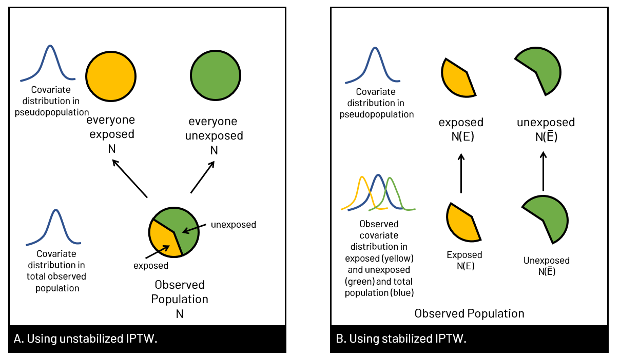

Unstabilized vs stabilized IPW | EPICODE

Figure 5. Panel A shows what happens in the pseudopopulation when we use unstabilized weights. We duplicate our N, creating 2 new populations with the covariate distribution of the entire observed population, but had everyone been exposed versus everyone unexposed. In B we apply the covariate distribution within strata of exposure, maintaining the same N. (E with a bar (macron) indicates unexposed).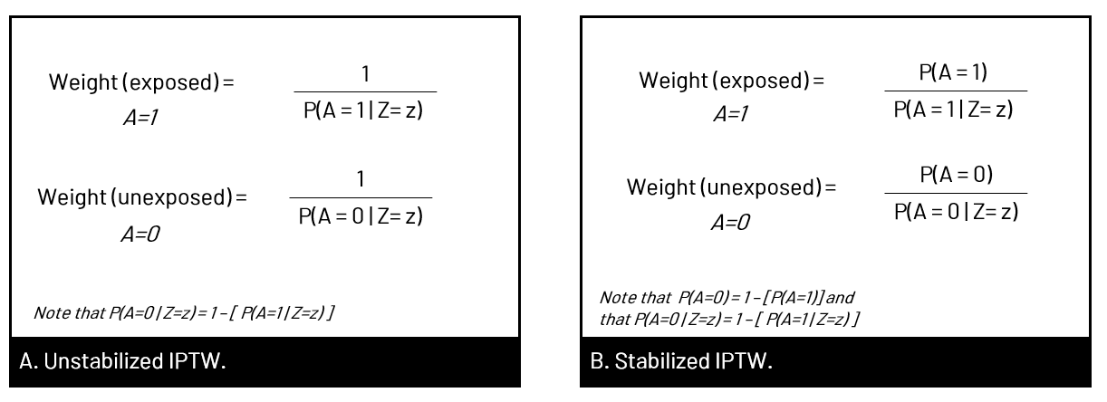

Figure 6. In Panel A we have the equation for unstabilized IPTW for exposed and unexposed, and in Panel B, the stabilized IPTW for exposed and unexposed. You'll see additional notes that show you that you can also calculate the weight components for unexposed by subtracting the exposed probabilities from 1. You'll see this used in our code below.

Unstabilized

Create a pseudopopulation 2x the size of our observed - one where everyone is exposed and one where everyone is unexposed.

Stabilized

Create a pseudopopulation maintaining the original population size, but we adjust the covariate distribution within each strata of exposure group by upweighting and downweighting people to match the overall covariate distribution.

You can see in Figure 5 versus Figure 3 that we are using different covariate distributions. With SMR where we match the covariate distribution of the exposed or unexposed group (whichever is target). This is why IPTW generates an average treatment effect while SMR generates an average treatment effect in the treated.

coding IPTW in SAS

******************************************
* Calculating IPTW
*****************************************;

&let data=<data>;
&let y=<outcome>;
&let x=<exposure>;
&let id=<id>;

*Estimate denominator - output a dataset with results of regression called denom, with the resulting probabilities stored in variable d;

proc logistic data=&data desc;
model &x = <covariates>;
output out=denom p=d;
run;

*Generate numerator for stabilized weights - output a dataset with results of regression called num, with the resulting probabilities stored in variable n - note that there is nothing on the right side of the equation because the numerator will simply be P(A=a), where a = observed exposure status;

proc logistic data=&data desc;
model &x=;
output out=num p=n;
run;

*Generate stabilized and unstabilized weights by merging the datasets with regression output (merge on the unique identifier in your dataset, &id);

data <newdata>;
merge &data denom num;
by &id;
if &x=1 then do;
uw = 1/d;
sw = n/d;
end;

*Remember we can use 1 - P(exposed) for the unexposed weight components;

else if &x=0 then do;
uw=1/(1-d);
sw=(1-n)/(1-d);
end;
run;

*Check the distribution of your IPTW - the mean should be 1. Is the sum for uw twice the sum of sw? why? is the range of uw greater than sw? why?;

proc means data=<newdata> mean sum min max;
var uw sw;
run;

*You can check to see if your exposure and covariates are associated in your new pseudopopulation (<newdata>);

proc logistic data=<newdata> desc;
weight sw;
model &x=<covariates>;
run;

*Now you can run your main analyses and apply the weights using the weight statement - use sw variable for stabilized weights, and use uw for unstabilized weights - you can use proc genmod, glm, logistic, etc. I'll show you below with logistic you can see now we're using &y and &x - and we don't need the covariates because the confounder -> x arrow is encompassed in the sw weight statement;

proc logistic data=<newdata> desc;
weight sw;
model &y = &x;
run;

coding IPTW in Stata

The approach to calculating IPTW is different in Stata than SAS. You'll be using the built in teffects command (reference manual [TE] here) and using options to specify IPTW.

Since using IPTW results in the average treatment effect overall, we'll use option ate (average treatment effect) instead of option atet (average treatment effect on the treated) that we use for SMR.

******************************************
* Calculating IPTW
*****************************************;

* Syntax for teffects statement

*teffects ipw (<outcome>) (<exposure> <covariates>), ate
*where <outcome> is your outcome variable, <exposure> is your exposure variable, and <covariates> is a list of your covariates to generate your weights.

*Example: Binary
*Outcome = lowbirthwt
*Exposure = maternalsmoke
*Covariates = maternalage nonwhite

*Use the teffects statement to generate your weights and then apply them in a logistic (default) model all in 1 step

teffects ipw (lowbirthwt) (maternalsmoke maternalage nonwhite), ate

*If your outcome is continuous, you can specify a probit model

*Example: Continuous
*Outcome = birthwt
*Exposure = maternalsmoke
*Covariates = maternalage nonwhite

teffects ipw (birthwt) (maternalsmoke maternalage nonwhite, probit), ate

* Syntax to manually create IPTW for binary exposure (treatment)
logistic treatment vars
predict p
gen iptw = 1/p if treatment==1
replace iptw=1/(1-p) if treatment==0

*To calculate stabilized IPTW, run tab treatment and use the proportions for X below
tab treatment
gen siptw = X/p if treatment==1
replace siptw = (1-X)/(1-p) if treatment==0

UPDATE: Feb 22 2021
If your treatment (exposure) is categorical you'll need to change things up a bit. I'm writing this blurb in response to a comment below, and in response to this topic coming up several times in just the past week!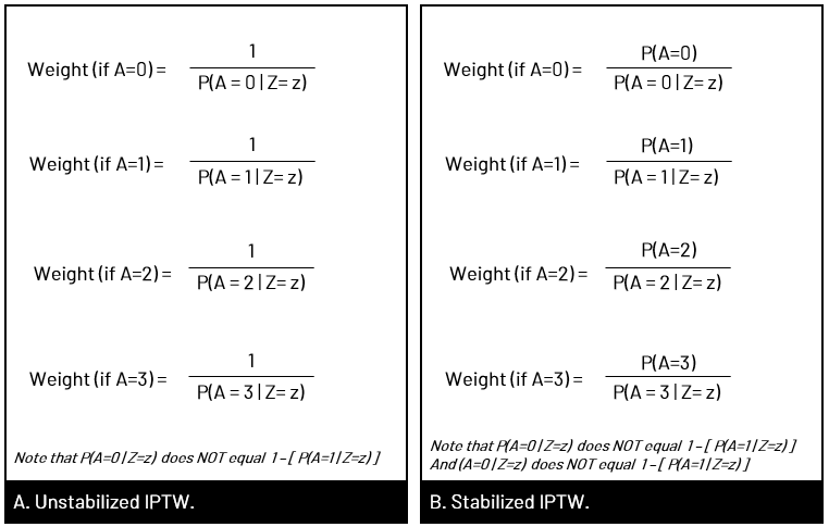

Figure 7. Calculating IPTW for a categorical A.

In your software of choice, you need to calculate the probability of being treated given your covariates, save those probabilities, and then assign the probability given each observations observed status.

In SAS, you can use code like the sample below (thanks, Paul!) which uses a generalized logit model for a treatment variable <treatment> with multiple categories.

The output data set will have probabilities for every value of treatment. For example, a person with treatment=1 will have values for treatment=0,1,2,3 so you need to do some more coding to tell the computer you only want the predicted value for treatment if treatment=treatment.

PROC LOGISTIC DATA=...;
MODEL treatment = vars / LINK=glogit;
OUTPUT OUT=denom_ipw P=d;
RUN;

In Stata, you can run mlogit to estimate the probability of <treatment> adjusted for variables <vars> and then use the postestimation commands, predict, to create a denominator variable for each value of treatment (0, 1, 2, 3). You use the option "outcome" to tell Stata this.

mlogit treatment vars
predict p0, outcome(0)
predict p1, outcome(1)
predict p2, outcome(2)
predict p3, outcome(3)

Then create your weight variable, iptw below.

gen iptw=.
replace iptw=1/p0 if treatment==0
replace iptw=1/p1 if treatment==1
replace iptw=1/p2 if treatment==2
replace iptw=1/p3 if treatment==3

If you want to create stabilized weights, you can run a tab to get the proportion in each category, and then calculate your weights. For example, let's say my groups are distributed as P(A=0)=0.6, P(A=1)=0.14, P(A=2)=0.2, and P(A=3)=0.06, I would make a stabilized iptw variable, siptw, below.

gen siptw=.
replace siptw=0.6/p0 if treatment==0
replace siptw=0.14/p1 if treatment==1
replace siptw=0.2/p2 if treatment==2
replace siptw=0.06/p3 if treatment==3

Download resources here, or get the most up-to-date versions on my GitHub

Calculating SMR and IPW - SAS - 2021 - EPICODE
File Size:	8 kb
File Type:	txt

Download File

Calculating SMR and IPW in Stata - 2022
File Size:	6 kb
File Type:	txt

Download File

Coding IPW and SMR in SAS and Stata - PDF for teachers
File Size:	551 kb
File Type:	pdf

Download File

Suggested citation

DeBarmore BM. “Coding IPW and SMR in SAS and Stata”. 2019. Updated 2021. Retrieved from http://www.baileydebarmore.com/epicode/calculating-ipw-and-smr-in-sas

About the author

Bailey DeBarmore is a doctoral student at the University of North Carolina at Chapel Hill studying epidemiology. Find her on Twitter @BaileyDeBarmore and blogging for the American Heart Association on the Early Career Voice blog.

15 Comments

Ken

2/5/2021 01:34:43 am

Hi Bailey. Really liked your post! I have a quick question: For IPTW, I wonder if the SAS codes can also be accommodated for an exposure with more than two groups. Say if x (exposure) can be 1, 2, or 3, then should we specify the stabilizing weight to be sw=(1-n)/(1-d) for x=1 (the referent group) and sw = n/d for x=2 and x=3 (the rest two groups)?

Bailey

2/5/2021 10:28:19 am

Hi Ken,

If your exposure=0,1,2,3 then you need to calculate the probability for each of these categories conditional on your covariates.

Use a generalized logit model (proc logistic with /link=glogit in the model statement) to do that. Your output dataset will have the predicted probabilities for exposure=0,1,2,3. For person i, if they have exposure = 2, then use Pr(Exposure=2|covariates) as their weight denominator. You would throw away the pred probabilities for that person where exposure=0, 1, 3. Once you have the predicted probabilities extracted based on their predicted values and observed exposure, divide 1 by the predicted value and fit your model with all treatment categories as independent variables. Shoutout to Paul Z for helping me answer your question.

-Bailey

2/5/2021 04:05:59 pm

Thanks Bailey and Paul for helping me on this! I found a SAS document that seems to suggest a similar solution to what you described: https://support.sas.com/resources/papers/proceedings/proceedings/forum2007/184-2007.pdf
However, it seems the weights created here are unstabilized weight? Thanks again for pointing me to the right direction.

Ann

2/26/2021 12:55:54 am

Hi Bailey,

Thank you for this detailed post!

I had a follow-up question about IPTW in STATA. You use the teffects ipw command which estimates the iptw and applies it to the outcome model all in one step. I was wondering if you'd be able to specify how to create iptw manually in Stata without using the teffects command. I ask because I'm using survey weighted data and my outcome model uses the svyset procedure which is incompatible with teffects.

2/26/2021 09:27:58 am

Great question, Ann! I've added some code to the Stata portion that specifies how to do this. Hope that helps!

2/26/2021 11:01:22 am

Thank you I just saw that! I did have a follow-up question, when you mention stabilizing the iptw, is it the same as normalizing the iptw? Performed as follows:

egen sum_weights = total(iptwt)
gen norm_weights = iptwt/sum_weights

2/26/2021 11:34:39 am

Hi Ann,

They're not quite the same. See above in the post where it talks at unstabilized versus stabilized weights. Stabilized weights have the probability of the exposure in the numerator.

Diego

4/9/2021 07:00:37 pm

Thanks for the information. It's really useful.I was wondering if the process is the same for IPW for attrition?

Thanks

5/24/2022 10:19:01 am

Hi Diego, thanks for the comment. The process would be the same or similar for IPW of attrition, you would replace your predictors of treatment with predictors of attrition. - Bailey

Joseph

4/28/2022 12:19:27 pm

Baily:
So glad I found your posting when searching the web to better understand IPTW. I am working in Stata, and would like to reproduce the output from teffects using a two step process that is required in SAS. You detailed above how to generate IPTW (and SIPTW). What would the code be to take that value and generate the same output as teffects?
Thanks!
PS: Typo in downloadable Stata code - header states SAS, should be Stata

5/24/2022 10:18:25 am

Hi Joseph, thanks for the comment (and the heads up about the typo - fixed now).

If you haven't already, I would compare the results from Stata's teffects to what you find in SAS to see if they differ. If they do, and you want to do them by hand, then I would recommend following the code for categorical exposure which uses mlogit, but instead use logistic and replace your numbers just for the two categories that you have.

-Bailey

Matthew

8/26/2022 12:26:43 pm

Hi Bailey, this is an amazing post about IPTW and just what I have been looking for.

I am a STATA user and want to know if there is a way to graphically show the level of balance in characteristics between say Drug A and Drug B before and after IPTW.

8/30/2022 10:47:27 am

You may find the command "tebalance" helpful. This article discusses it (scroll down until you see the balance plots).

https://www.stata.com/stata14/treatment-effects-balance/

Selina

2/6/2023 05:37:32 am

Hi Bailey,

Thank you for this post. I already used your SAS code and have a question regarding the distribution of uw and sw.
The following means I got: uw=1.997 and sw=0.999. The range of uw is greater than sw.

You wrote in the code: " ... the mean should be 1. Is the sum for uw twice the sum of sw? why? is the range of uw greater than sw? why?"
Are there some reasons for the distribution of uw/sw I got?

Val

9/14/2023 04:36:08 pm

I have data where the unexposed group is much larger than the exposed group, so the SMR weights are very small for the unexposed group. Is it valid to normalize the SMR weights for the unexposed group to have a mean of 1 (i.e. divide the SMR weights by the mean for the group). That makes the sum of all the weights similar to the total study population, but does it still mean that I am estimating ATT?

Your comment will be posted after it is approved.